I3 Power Sensor – User Manual (PDF download)
Overview
First time quick start
Sensor variants
Interface options and requirements
Starter kit contents
System installation
Voltage sensor installation
Current sensor installation
Installation considerations
Starting the sensor
Basic configuration
Using the graphical web interface
Resetting the sensor
Setting the IP configuration of the sensor
Setting cable conductor configuration
Advanced configuration
Using the FTP interface
Using the Telnet command line interface
Using the Lua scripting interface
Using and configuring the IEC 60870-5-104 protocol
Updating sensor software
Efficient mass reconfiguration of sensors
Measuring voltages
Measurement configurations
Voltage signal interfacing
A note on spread capacitances
Guide for setting up voltage cross talk cancellation on the I3 sensor
Troubleshooting
Appendix
Web interface menu structure
Conductor models
Telnet commands
Overview
The I3 Power Sensor system is a sensor system designed for measuring voltage, current and all derived quantities for multiple conductors in low- or medium voltage installations.
The I3 system is designed to be fully self-contained, including high level post-processing of measurements, remotely operated, easy to install, easy to use, and virtually maintenance free.
The complete system consists of a capacitive voltage interface and integrated magnetic current sensors. Once installed, the system is configurable through various interfaces, including remote options.
First time quick start
- Attach the sensor to a PoE switch on your network.
- Determine the assigned IP address of the sensor either by looking into your allocation table in your network switch/router/firewall or by use of the Jomitek Device Locator software which can be found here (Download .exe file | Download .zip file).
- Open your browser and go to the IP address of the sensor.
- Explore the graphical web interface.
Sensor variants
The basic I3 sensor allows for current measurement in up to four phases with a single phase voltage measurement. The more advanced I3+ sensor allows current measurements in up to four phases with voltage measurements in three phases with one additional (null) phase.
Additionally, both the basic I3 and the I3+ sensors come in two physical sizes intended for cable diameters of up to 60 mm and up to 80 mm respectively.
Interface options and requirements
The sensor uses a single RJ45 connector for both communication and power supply. The sensor should be powered by either Power over Ethernet (PoE) or through direct 24V or 48V DC power supply into the Ethernet cable.
When the sensor is connected, it can accessed through a graphical web interface, IEC 60870-5-104 protocol, FTP, or a Telnet or Lua command line interface.
Starter kit contents
The starter kit will help you build a test setup for evaluating the functionality and performance of the I3 sensor system.
- Current sensor
- 1× small I3+ sensor (60 mm cable diameter)
- 1× large I3+ sensor (80 mm cable diameter)
- Voltage sensor
- 2× Capacitive voltage measurement interface with CEE connector
- 2× CEE adapter
- Installation accesories
- Cable ties with fastening tool
- Adhesive rubber patches
- Adhesive velcro patches
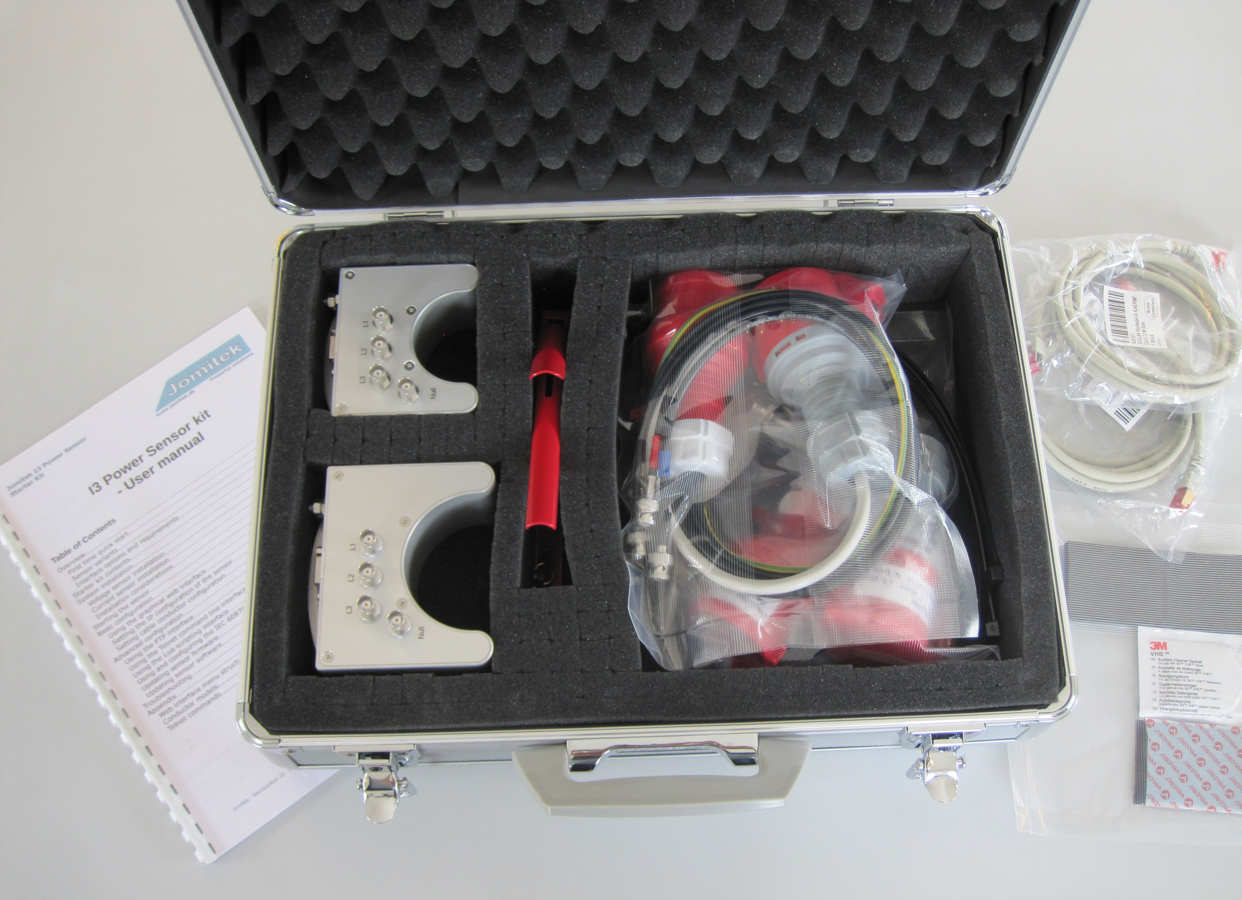
Figure 1: The I3 Power sensor starter kit.
System installation
Installation of the I3 sensor system is simple and requires no calibration for current measurements, and optional calibration for voltage measurements, depending on accuracy needs. Simply attach the I3 current sensor to the cable to be measured. Connect the capacitive voltage measurement interface connector(s) and finally attach the Power over Ethernet cable. The installation procedure is described in detail in the following sections.
Voltage sensor installation
The starter kit includes two capacitive voltage measurement interfaces for voltage sources below 500V nominal peak. The measurement interface uses built-in capacitors and can therefore be directly connected between a voltage source with a CEE plug and the BNC connectors on the I3 sensor. If your voltage source does not use a CEE plug, you can use the included CEE adapter to convert to any other connector type you may wish to use in stead.
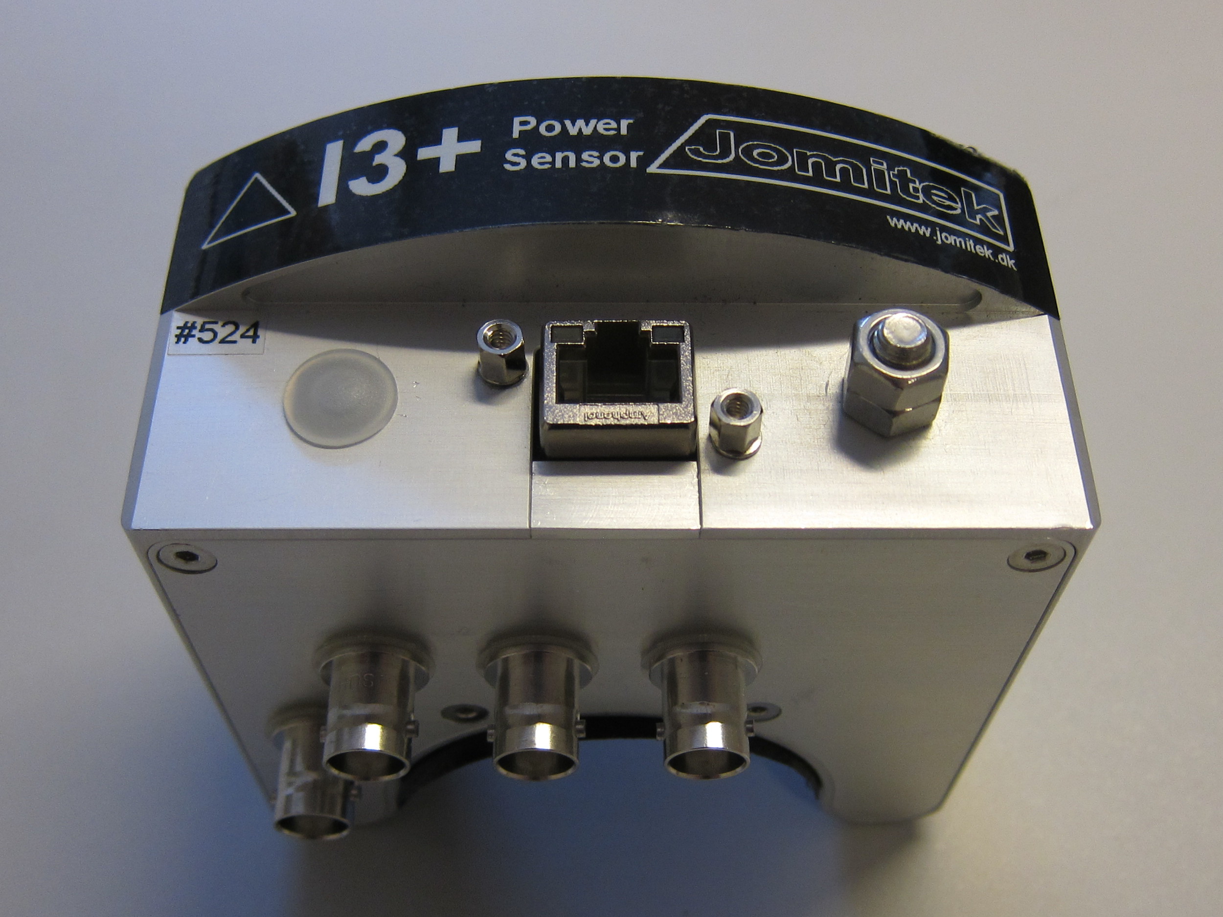 Figure 2: Front and bottom view of the I3 sensor showing the PoE port, grounding point and voltage measurement BNC connectors. |
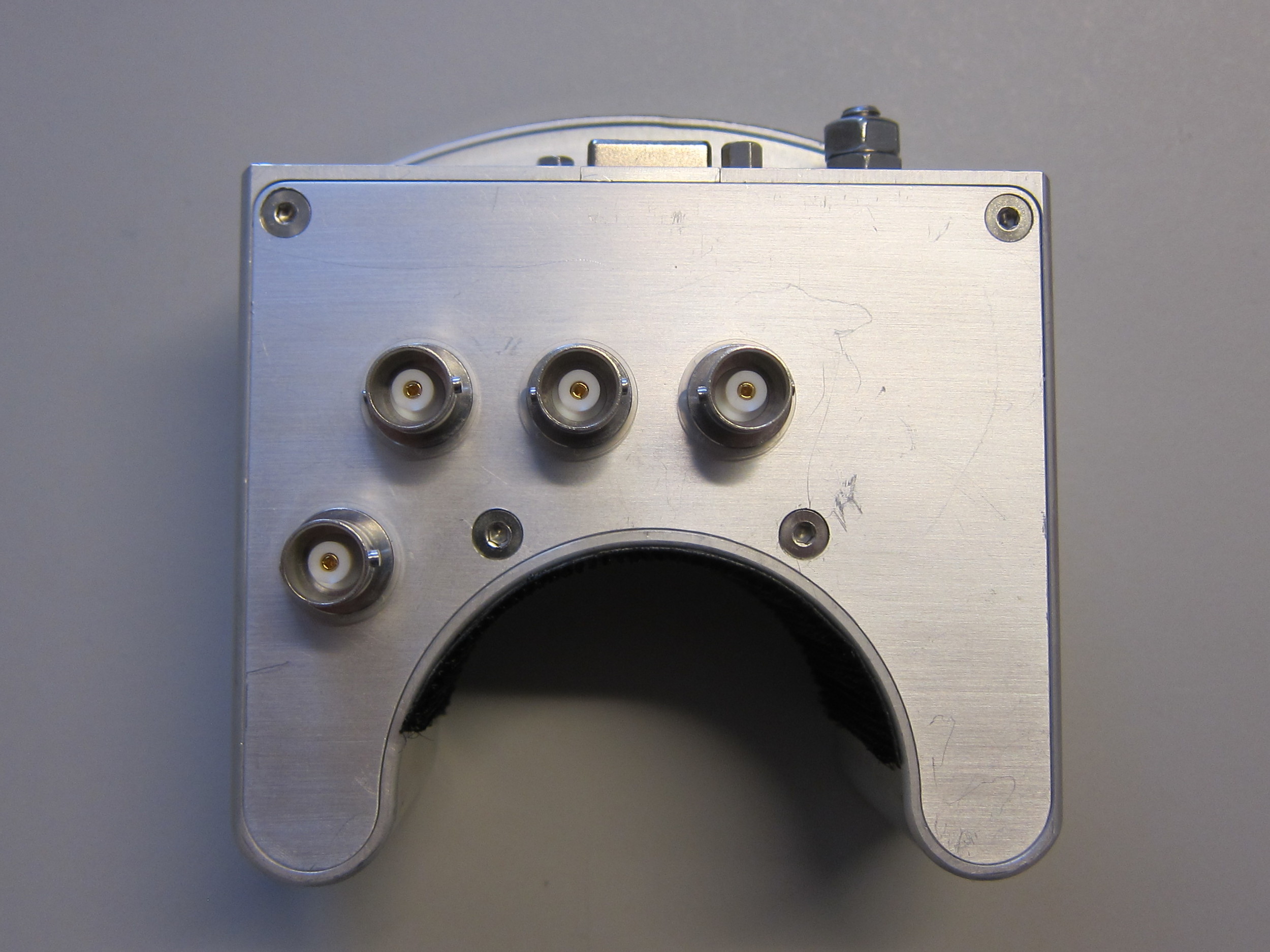 Figure 3: Voltage measurement BNC connectors starting from the lower left going up to the right: Null, L3, L2, L1. |
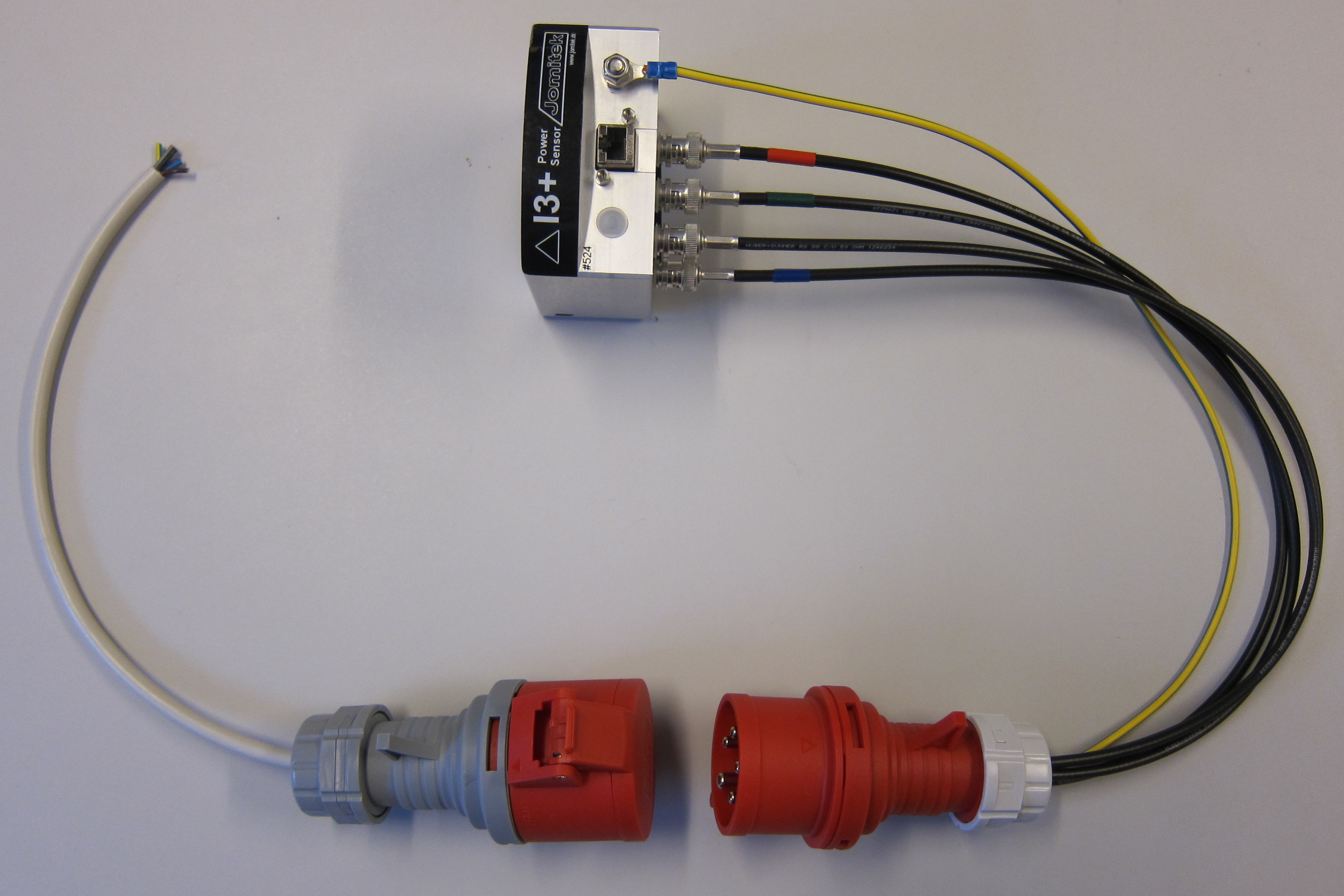 Figure 4: Capacitive voltage measurement interface attached to the I3 sensor. The CEE adapter is shown to the left. |
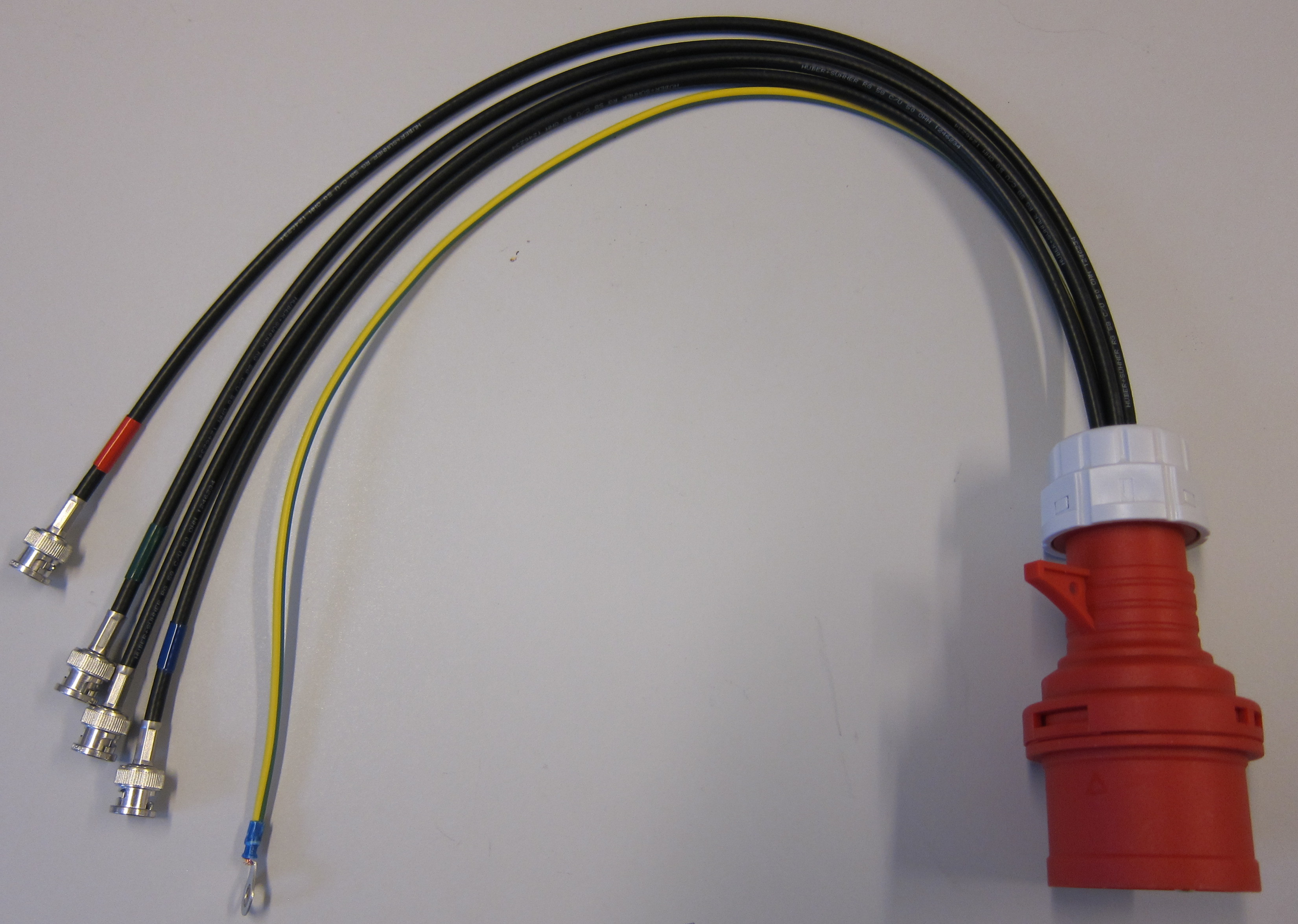 Figure 5: CEE adapter for use with the capacitive voltage measurement interface. |
The CEE adapter is intended for use when your voltage source does not use a CEE plug. Attach your own connector to the adapter, and attach the adapter to the capacitive voltage measurement interface. Refer to the voltage phase identification color codes listed in table 1 for correct wiring of your own connector.
| Electrical potential | Capacitive voltage measurement interface (wire color) | CEE adapter (wire color) |
| Ground | Green/yellow | Green/yellow |
| Null | Blue | Blue |
| L1 | Red | Brown |
| L2 | Green | Black |
| L3 | Black (no label) | Grey |
Table 1: Electrical phase color coding for voltage measurement.
Current sensor installation
Place the current sensor on the cable and secure it with the provided cable ties as shown. The sensor must be mounted such that voltage BNC connectors are facing down.
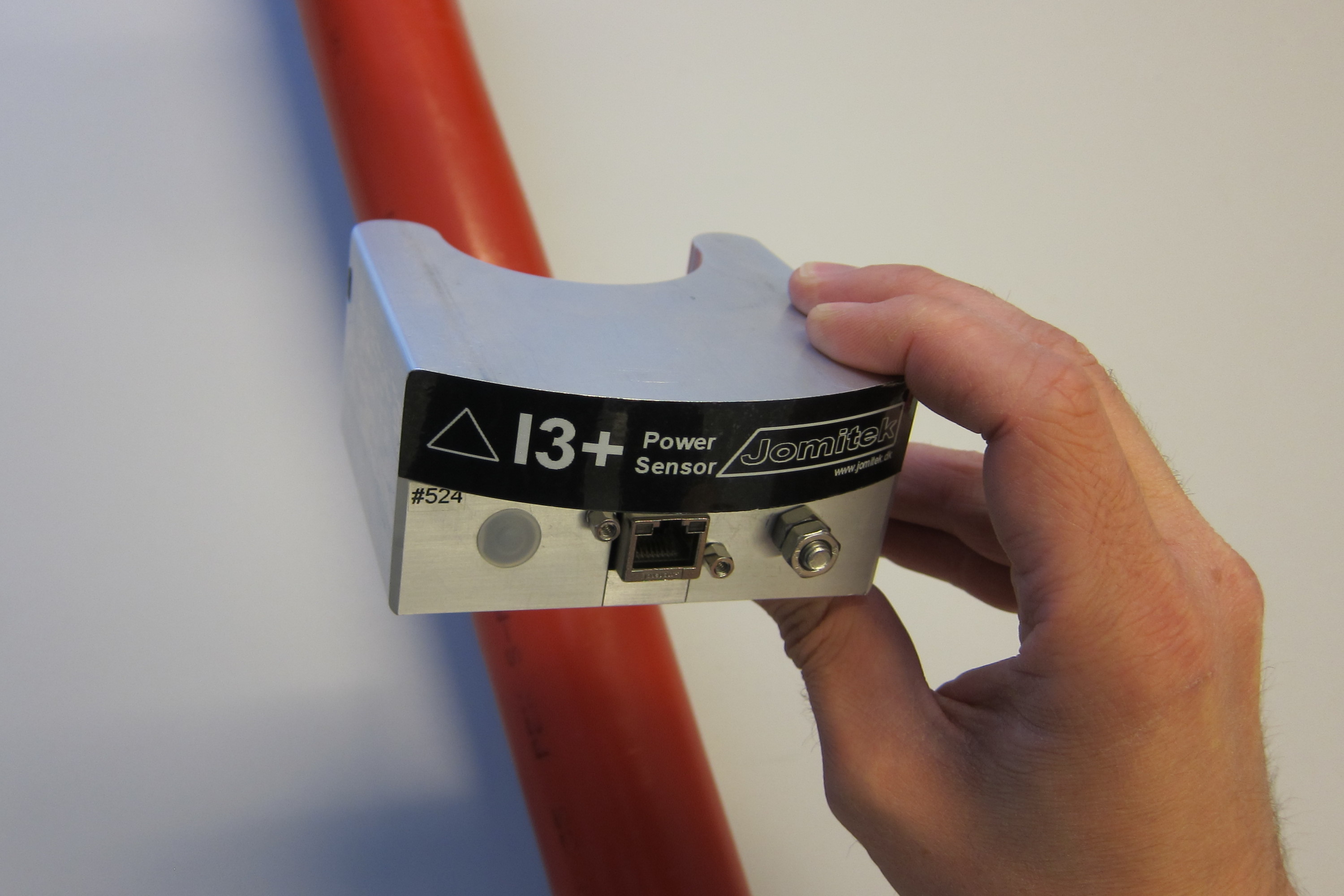 Figure 6: Place the sensor on the cable to be measured. |
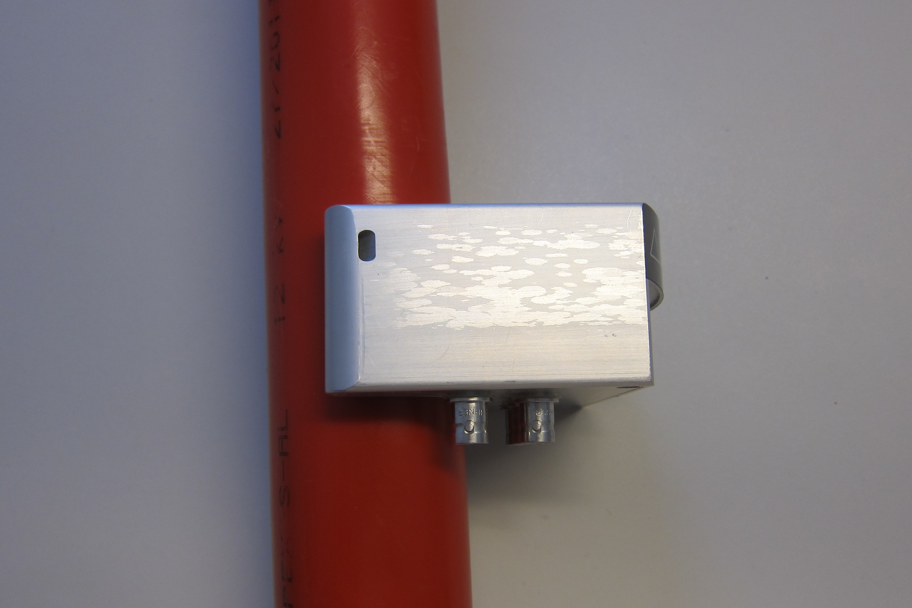 Figure 7: Make sure that the sensor is mounted such that the voltage BNC connectors are facing down. |
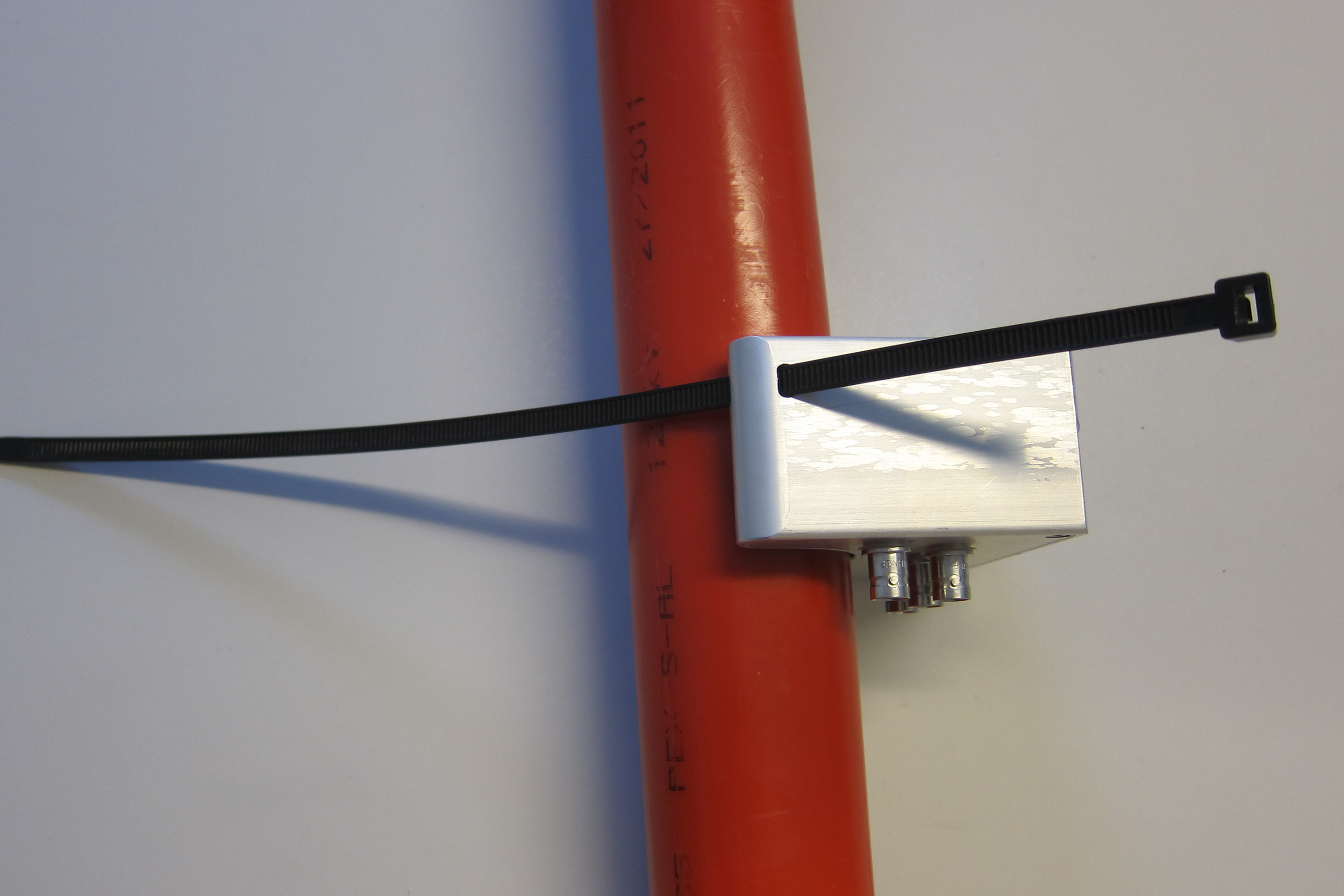 Figure 8: Insert the cable tie in the cutout on the sensor. |
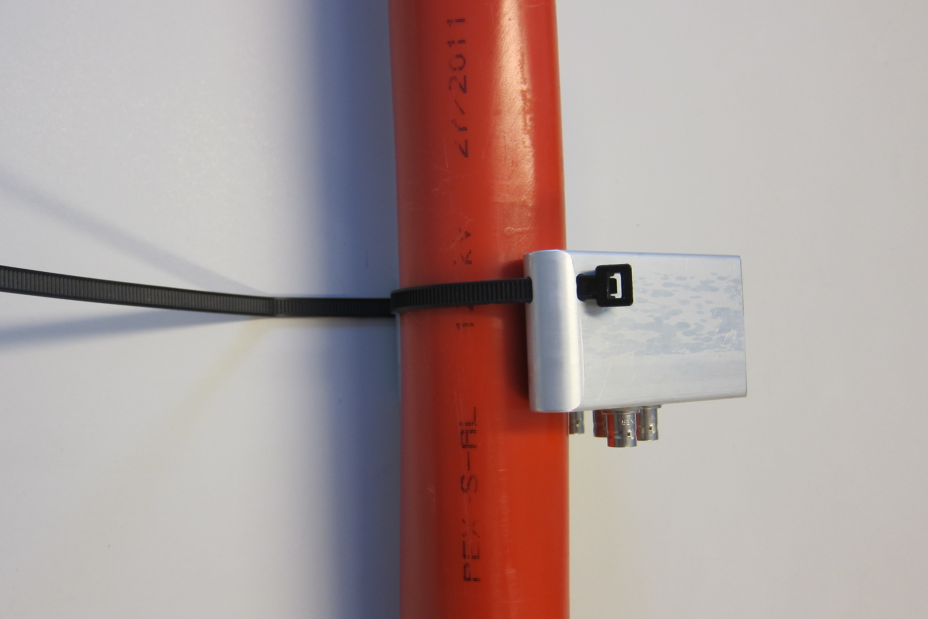 Figure 9: Wrap the cable tie around the cable and thread it through the cutout on the opposite side of the sensor. |
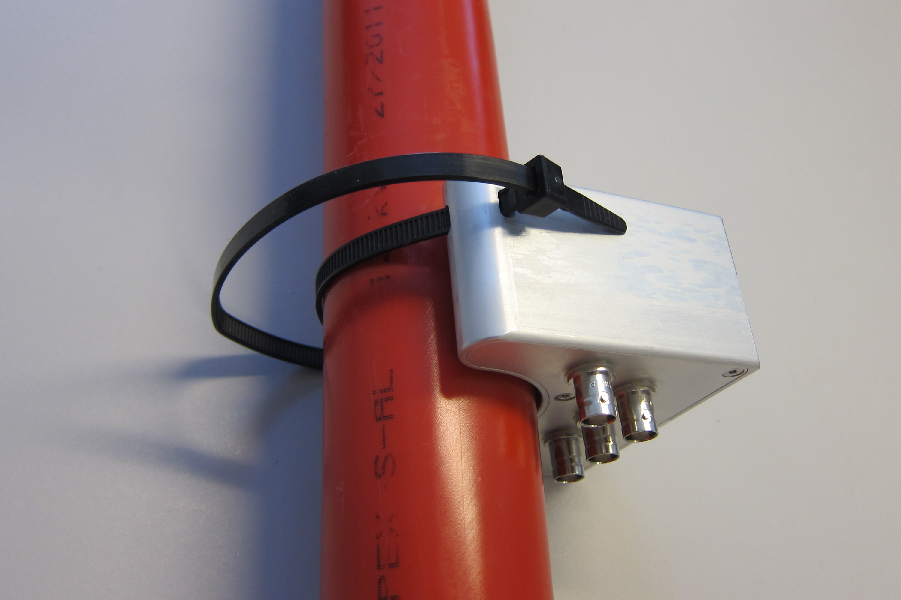 Figure 10: Complete the cable tie connection. |
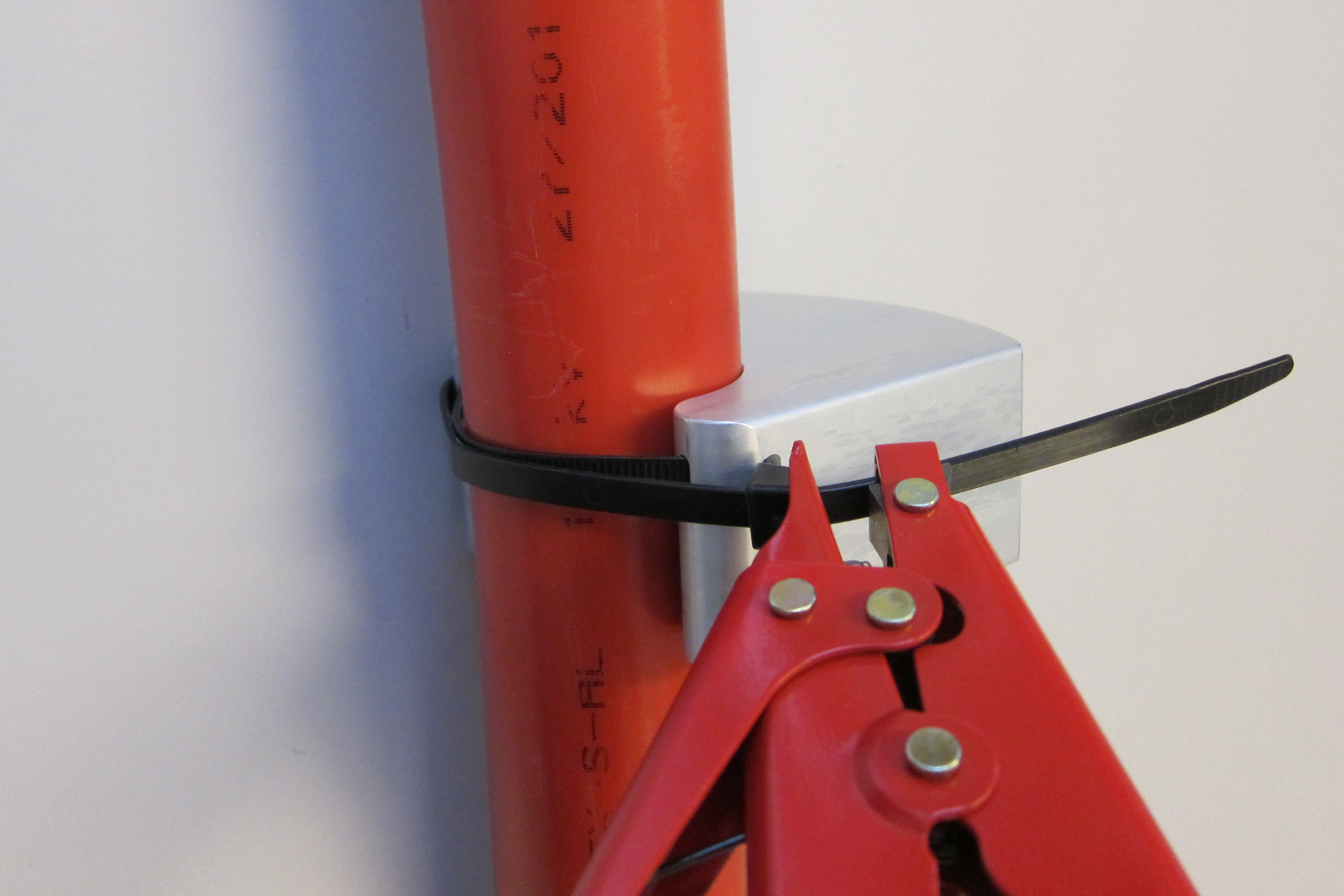 Figure 11: Use the provided tool to tighten the cable tie. |
The sensor can be lined with the included adhesive rubber or velcro patches if the cable diameter is significantly smaller than the sensor U-shape. It is recommended to always use a cable tie to complete the sensor installation.
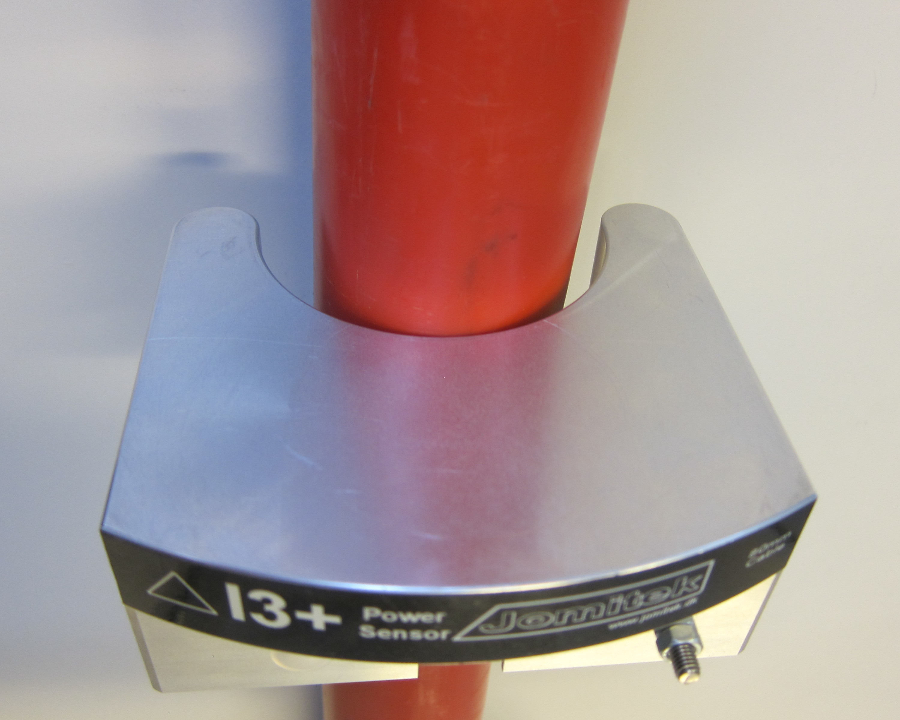 Figure 12: The cable diameter is too small for the sensor. A good fit is not possible. |
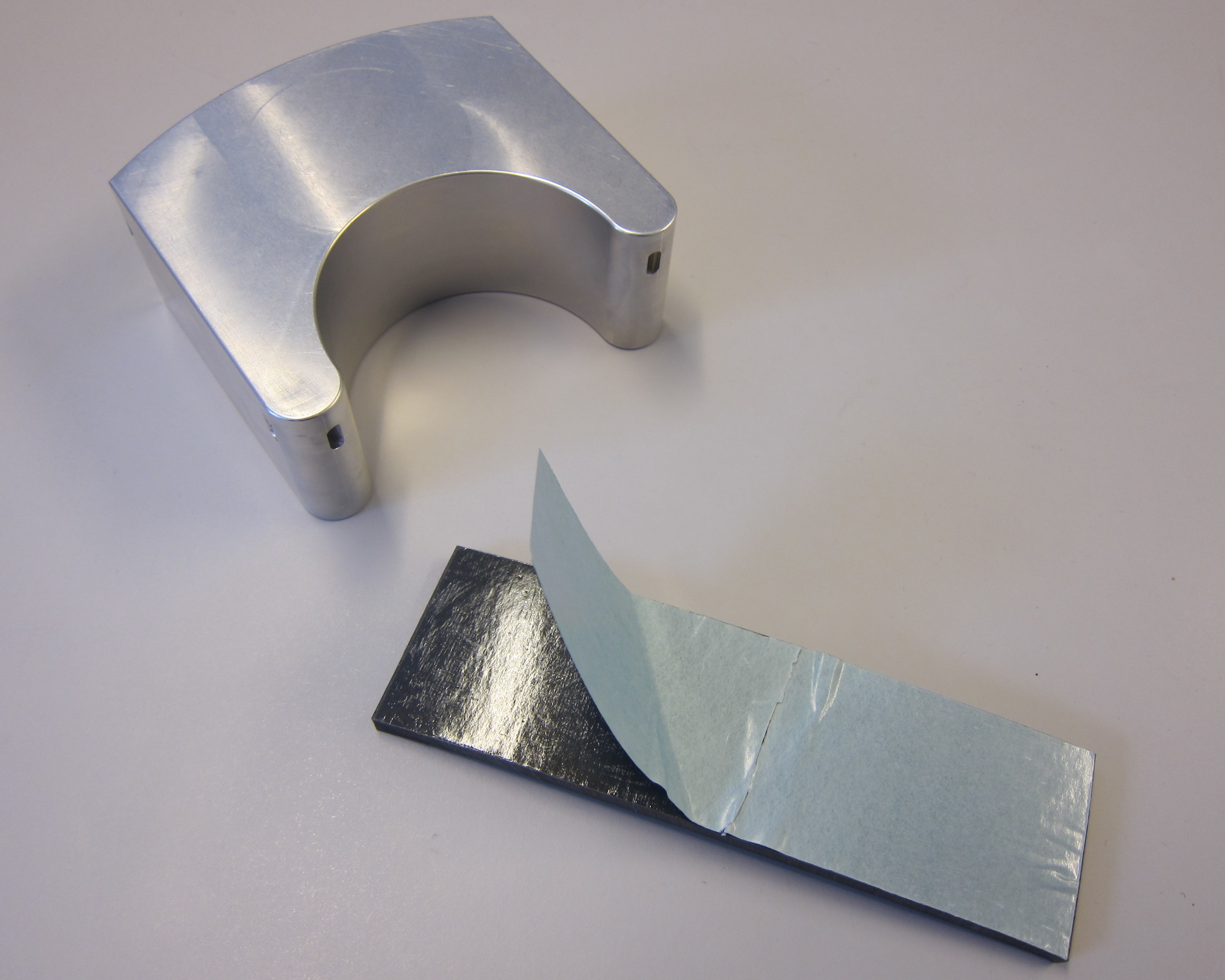 Figure 13: Use the adhesive rubber patch to line the sensor. |
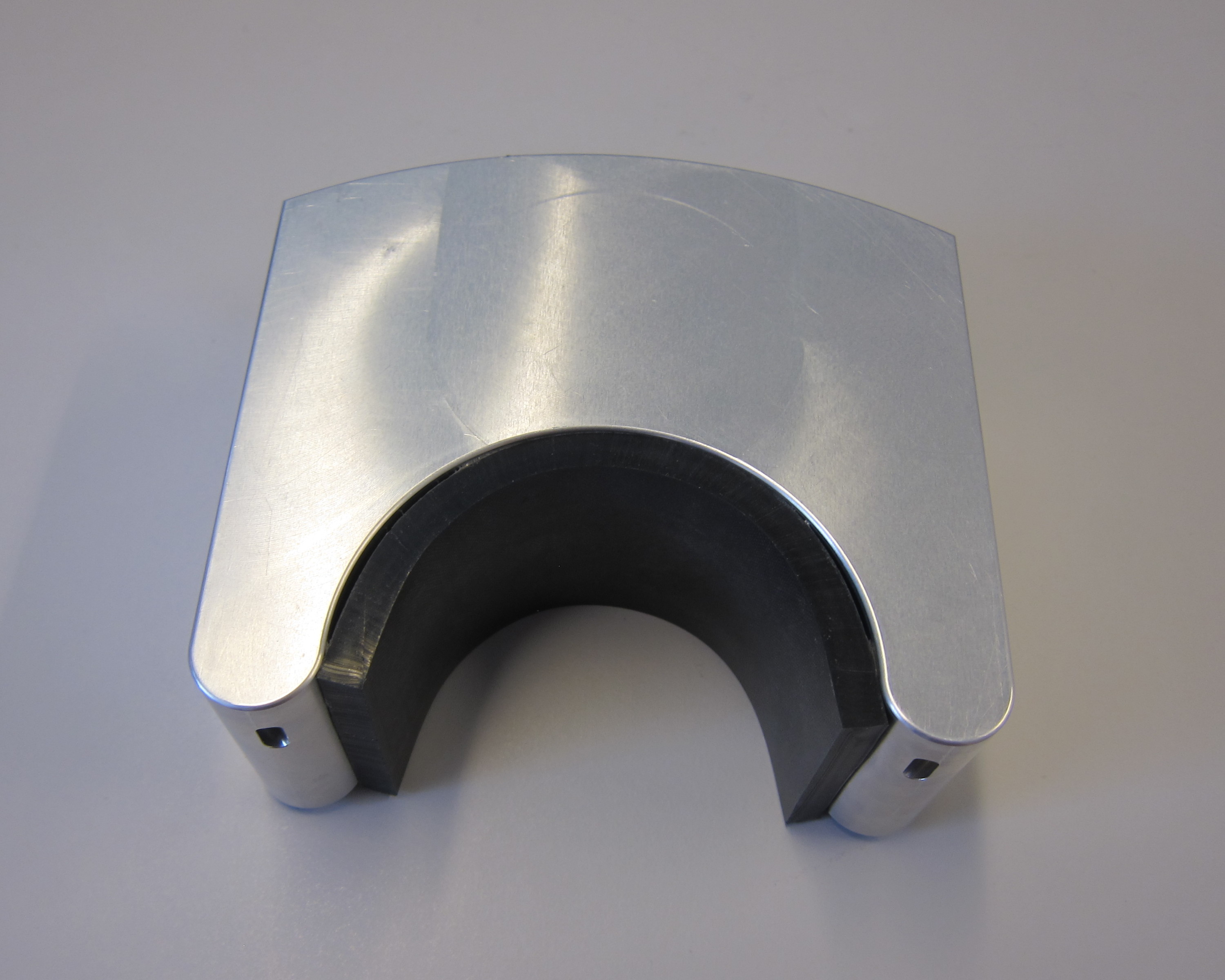 Figure 14: Adhesive rubber patch applied to the sensor in order to reduce the diameter. |
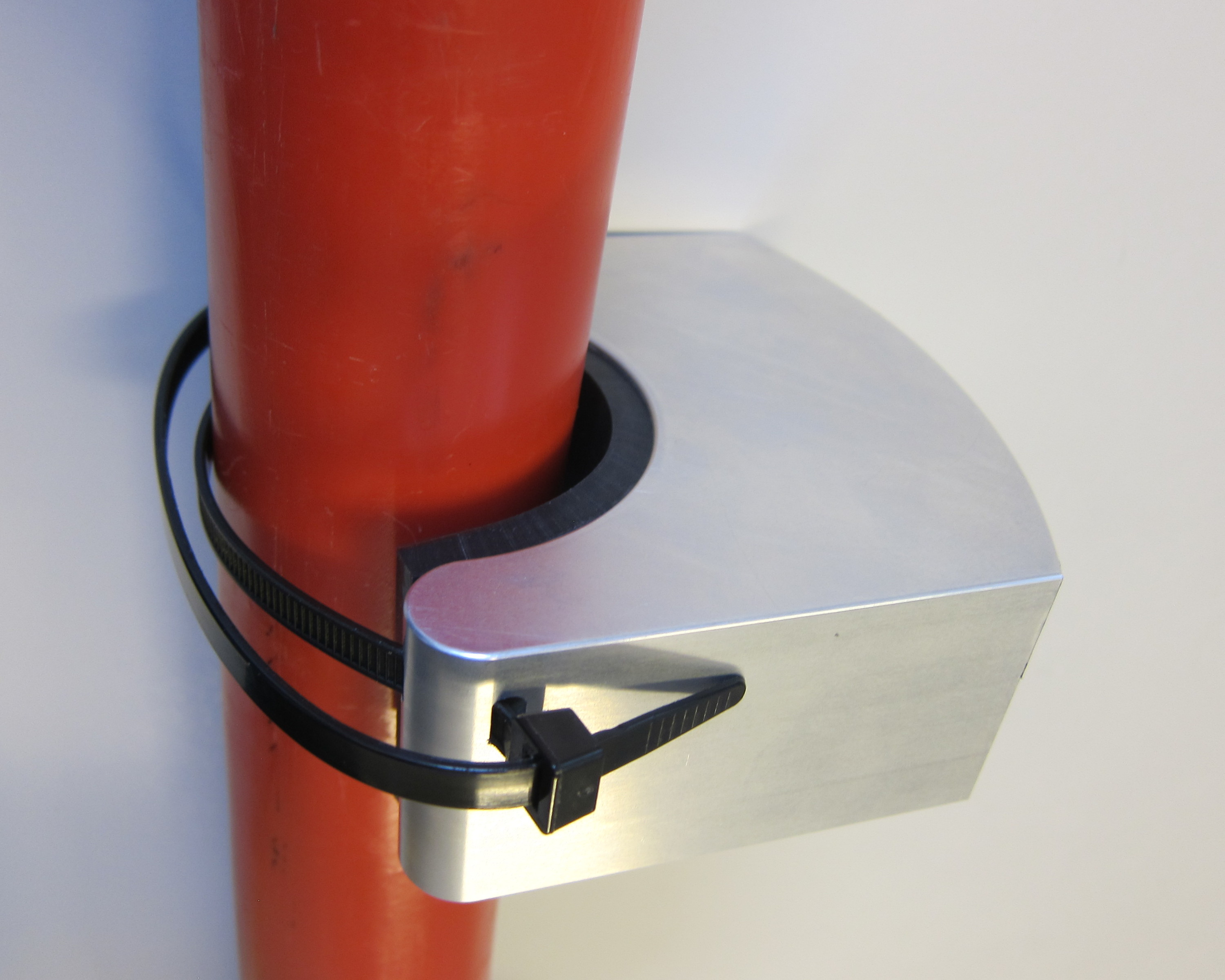 Figure 15: The cable and sensor diameters match, and a secure fit is now possible. |
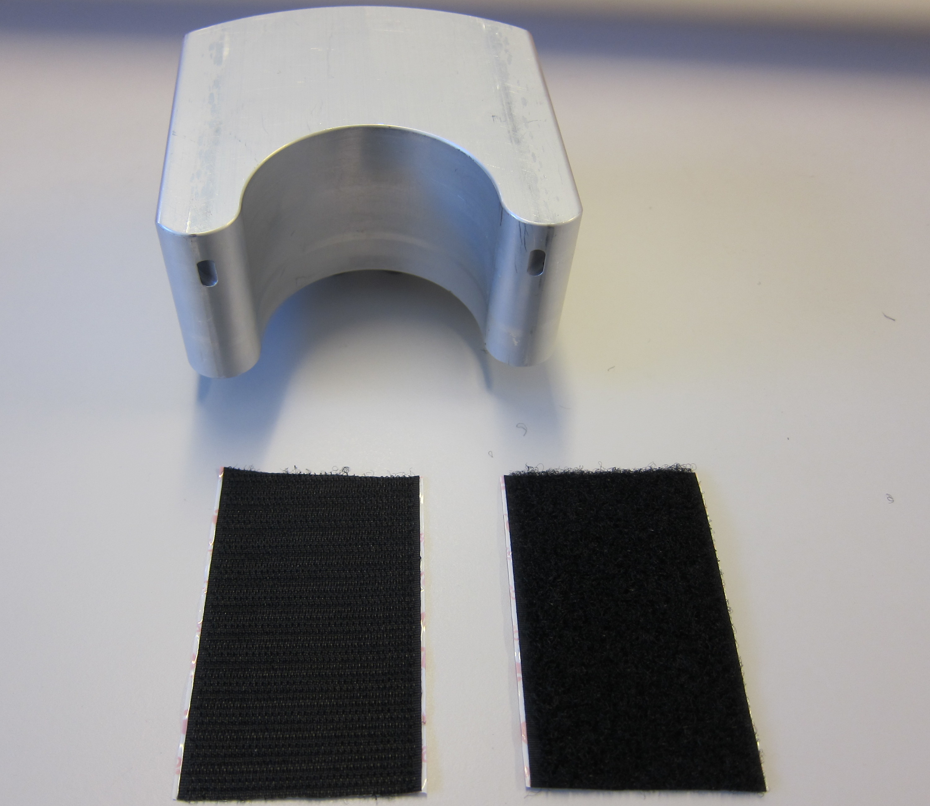 Figure 16: Adhesive velcro patches can be used in stead of the rubber patches. |
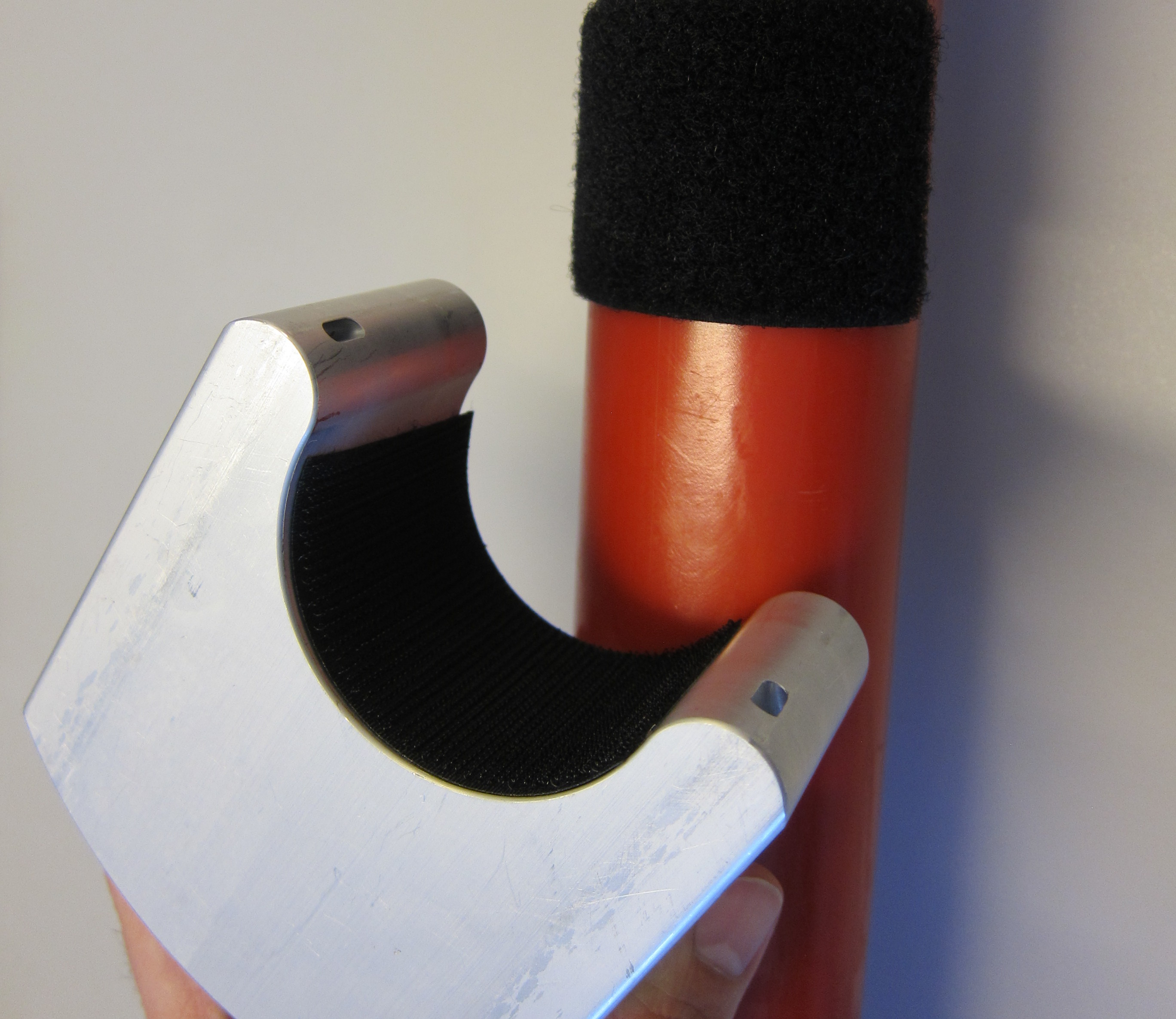 Figure 17: Always use a a cable tie to finish the installation, even when using velcro. |
Attach the grounding cable on the front of the sensor, then plug in the voltage cables to the BNC connectors at the bottom of the sensor as shown in figure 18.

Figure 18: Attach the grounding cable and the voltage BNC connectors.
Installation considerations
The I3 sensor works by measuring the magnetic field generated by the current running in the cable. For best sensor performance, it is important to minimize magnetic disturbances close to the sensor. In general, this means that iron and other ferromagnetic materials should be avoided within 5-10 cm of the sensor box.
When building a laboratory setup for testing and evaluation, please note that the return conductor in a current loop should be kept as far away from the sensor as possible. The sensor is designed to be particularly weather resistant when mounted with the bottom part facing down.
Starting the sensor
The sensor will turn on and start up automatically when an Ethernet cable with Power over Ethernet (PoE) is plugged in. The sensor measurements are available through a web interface, as well as the IEC 60870-5-104 protocol.
The sensor is per default configured to receive an IP address from a DHCP server, but will fall back to a default IP address if no DHCP server is present on the network.
The Jomitek Device Locator software tool which is available here (Download .exe file | Download .zip file) can be used to identify I3 sensors on your network.
Basic configuration
All basic sensor configuration can be done through the web interface which is also used to provide quick and easy access to all measurements.
Using the graphical web interface
The web interface can be accessed in a web browser by navigating to the IP address of the sensor.
The interface menu system consists of a hierarchical folder structure which gives access to all sensor settings and measurements. The folder structure provides a graphical representation of the text based configuration files stored in the conf folder in the internal memory of the sensor.
This means that updating a setting in the web interface will update the corresponding configuration file in the conf folder and vice versa.
Hovering the mouse pointer above a setting will provide a helpful tooltip with further information as shown in figure 19.
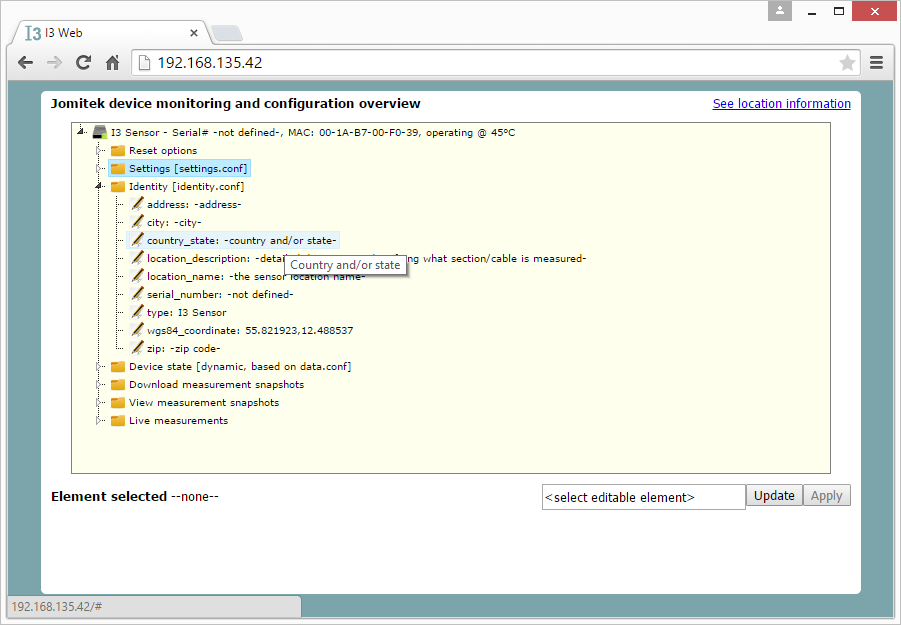
Figure 19: Web interface shown in browser. Notice the tooltip being shown when hovering the mouse pointer over a setting.
A setting is updated in four steps (refer to Figure 20):
- Select the setting to be updated.
- Edit the value.
- Click the ‘Update’ button.
- Click the ‘Apply’ button.

Figure 20: Updating the value of a setting in the web interface.
Multiple updates can be sent to the sensor by going through steps 1-3 for each setting change, and then applying all updates in a single step by executing step 4 once.
Viewing a measurement in the web interface is accomplished in a similar way. Select the measurement you want to view, and it will be shown in the graph window below the menu window. You can use the ‘Close graph window’ button to clear the graph window when you are done.
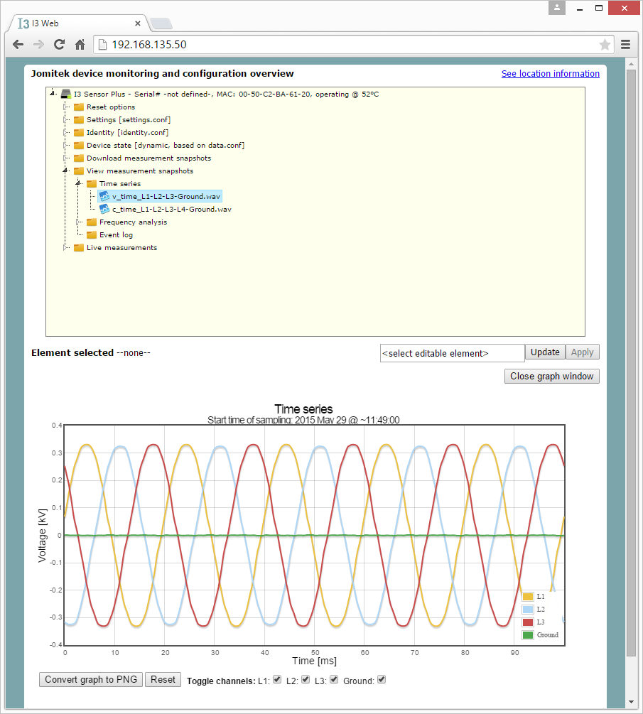
Figure 21: Viewing a measurement in the web interface.
Please refer to the appendix for a complete description of the web interface menu structure.
Resetting the sensor
The sensor requires a reset for changes in IP-configurations to take effect. The reset can performed by physically removing power (i.e. removing the Power over Ethernet connector), or by a software reset performed through the web interface. This is illustrated in figure 22.
If the IP-configuration was changed to use DHCP, the sensor might have a new IP-address when starting up after a reset, and it might be necessary to use the Jomitek Device Locator program to find it on the network.
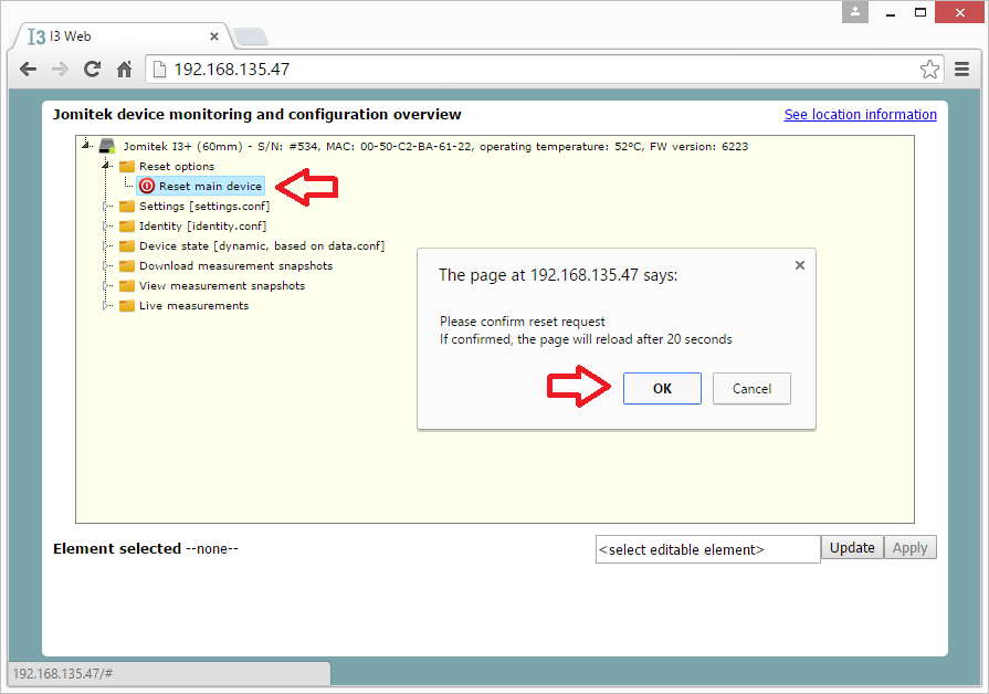
Figure 22: To perform a sensor reset through the web interface go to Reset options ⇒ Reset main device and click ‘OK’ to the message box.
Setting the IP configuration of the sensor
Set the IP configuration of the sensor through the web interface by navigating to Settings ⇒ tcpip. The IP address, gateway and subnet can be set manually if the option to use DHCP is set to ‘false’.
The sensor must be restarted after making changes to the IP-configuration in order for the changes to take effect.
Setting cable conductor configuration
The I3 sensor can measure different cable types ranging from simple one-conductor cables to more complicated three- or four-conductor cables. In the web interface, navigate to Settings ⇒ i3 ⇒ estimator ⇒ estimator_mode to select the appropriate conductor configuration for the cable being measured.
Refer to the appendix for a full list of available conductor models.
Advanced configuration
More advanced configuration and debugging can be achieved using the either the FTP, Telnet or Lua interfaces.
Using the FTP interface
The internal memory on the I3 sensor can be accessed via the FTP protocol on port 21. Use an FTP client program (e.g. FileZilla) and sign in with username ‘service” and password ‘service1234‘.
When connected you will have access to three folders.
- The conf folder where configuration files and scripts are stored.
- The software_update folder where software update files can be uploaded.
- The log folder where various log files are placed by the sensor system.
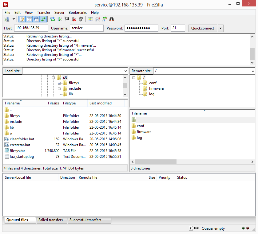
Figure 23: FTP connection to the I3 sensor shown with the FileZilla FTP client.
Using the Telnet command line interface
For advanced maintenance and debugging tasks, the I3 sensor can be accessed and configured via a limited command line interface using Telnet. This interface is accessed by connecting to the sensor’s IP address on port 23 using a standard Telnet client. It is recommended to use Putty which is open source and free to use.
Be sure to enable the “Implicit CR in every LF” and “Implicit LF in every CR” options when configuring Putty.
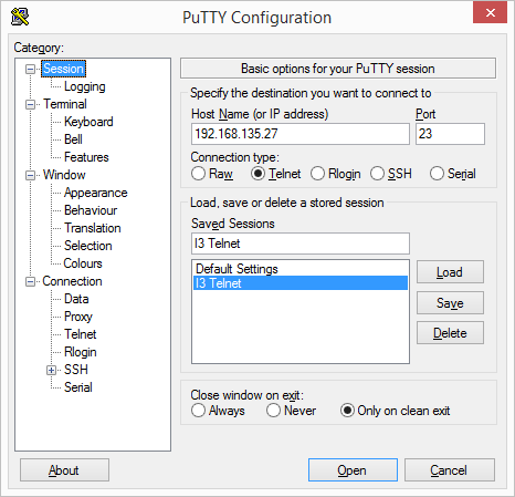 Figure 24: Putty Telnet Session configuration. |
 Figure 25: Putty Telnet Terminal configuration. |
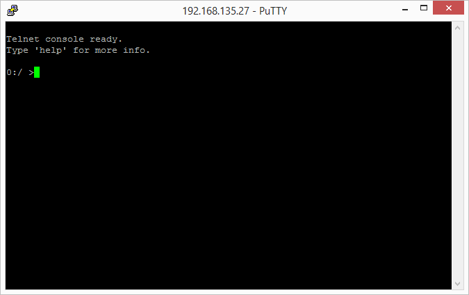
Figure 26: The Telnet command line interface.
Refer to the appendix for a full list of currently available Telnet commands.
Using the Lua scripting interface
The I3 sensor features an embedded scripting engine running the Lua1 programming language. This scripting engine allows for advanced configuration and dynamic re-configuration of the sensor.
Connect to a Lua command line prompt by connecting to the sensor’s IP address on port 2840 using Putty.
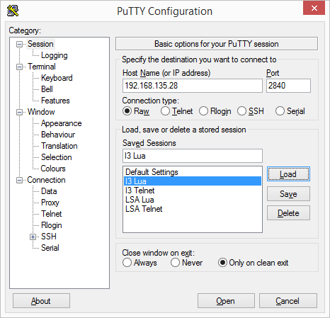 Figure 27: Putty Lua Session configuration. |
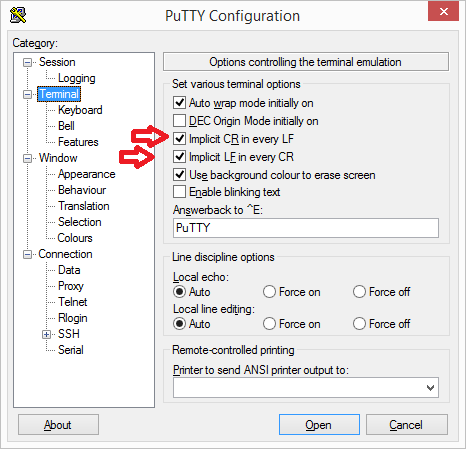 Figure 28: Putty Lua Terminal configuration. |
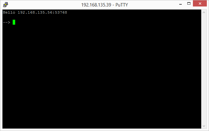
Figure 29: The Lua command prompt.
The Lua interface is intended for advanced configuration and debugging and should only be used by experienced users.
Using and configuring the IEC 60870-5-104 protocol
The IEC 60870-5-104 (abbreviated “104”) application layer protocol can be used for transmitting sensor data from the sensor to a SCADA system or another data-aggregation device implementing the 104 protocol. The TCP/IP protocol suite is used to ensure reliable data transfer. Additionally, the 104 protocol supports message sequencing on the application layer. A 104 client connects to the IANA assigned TCP port 2404 is available on the sensor.
The sensor allows very flexible configuration of the protocol settings, and of the data points. The data points can be transmitted based on a variety of triggers, including on-change, periodic, on manual request, or using interrogation commands requesting a larger set of data. The sensor can be configured to use all features defined in the IEC 104 standard, or the sensor can use a small subset for simpler applications.
The 104 protocol settings are found in the settings.conf file under the “iec104” section. These shall match the protocol settings defined in the SCADA client, and must be in compliance with the IEC standard. Interoperability requirements can be documented by a 104 client by filling out Chapter 9 in the IEC 104 standard. An overview of the parameters defined in the sensor are listed in table 2.
| Setting | Meaning | Default value |
| t1 | Time-out of send or test APDUs. | 16 |
| t2 | Time-out for acknowledges in case of no data messages, t2<t1. | 11 |
| t3 | Time-out for sending test frames in case of a long idle state. | 21 |
| k | Maximum difference receive sequence number to send state variable. | 8 |
| w | Latest acknowledge after receive w I format APDUs. | 12 |
| common_address | IEC 104 address of sensor. | 1 |
| background_scan | Interval in seconds between transmission of digital data points. | 1800 |
| cyclic | Interval in seconds between transmission of analogue data points. | 600 |
| scan | Data change scan interval in milliseconds for sending event-triggered data. | 500 |
| clock_validity | Time-tagged client commands validity period in seconds. | 600 |
| redundancy | Max number of redundant connections as defined by IEC 104. | 2 |
Table 2: IEC-104 parameters.
Three .csv files are used to map internal sensor measurements to data points accessible by an IEC 104 client. A macro enabled Excel file is used to generate these .csv files, and all changes to the data mapping should be applied in the Excel file. There are three sheets in the Excel file, and each generate one .csv file. The sheets are called “iec104_analogue”, “iec104_digital” and “iec104_commands”, which define analogue and digital measurement mapping to the IEC 104 protocol. An example snapshot of the “iec104_analogue” sheet is shown in figure 30.
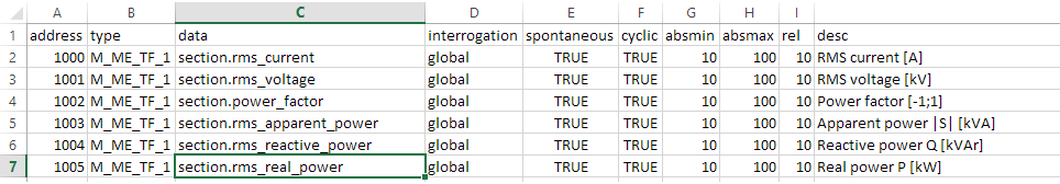
Figure 30: iec104_analogue.
Description of columns:
- address The address of the data point, [1-65535].
- type The IEC 104 type (see interoperability list in IEC 60870-5-104 chapter 9).
- data Internal sensor variable name.
- interrogation The interrogation group this data point belongs to. Can be “global” or “groupX” where X is in the range [1-16].
- spontaneous Set to true if data point should be transmitted on change.
- cyclic Set to true if data point should be sent periodically.
- absmin Minimum absolute change in data value to trigger spontaneous transmission. This is useful for avoiding sending a data point too often when the value is low.
- absmax Maximum absolute change in data value to trigger spontaneous transmission.
- relRelative change in percent of the data value to trigger spontaneous transmission. For example, setting rel = 10 for a data point with value 500 triggers transmission at 450 or 550.
- desc A short description of the data point and unit. The description will be used as a tooltip in the web interface.
Refer to figure 31 for a graphical example of the transmission thresholds absmin, absmax and rel.
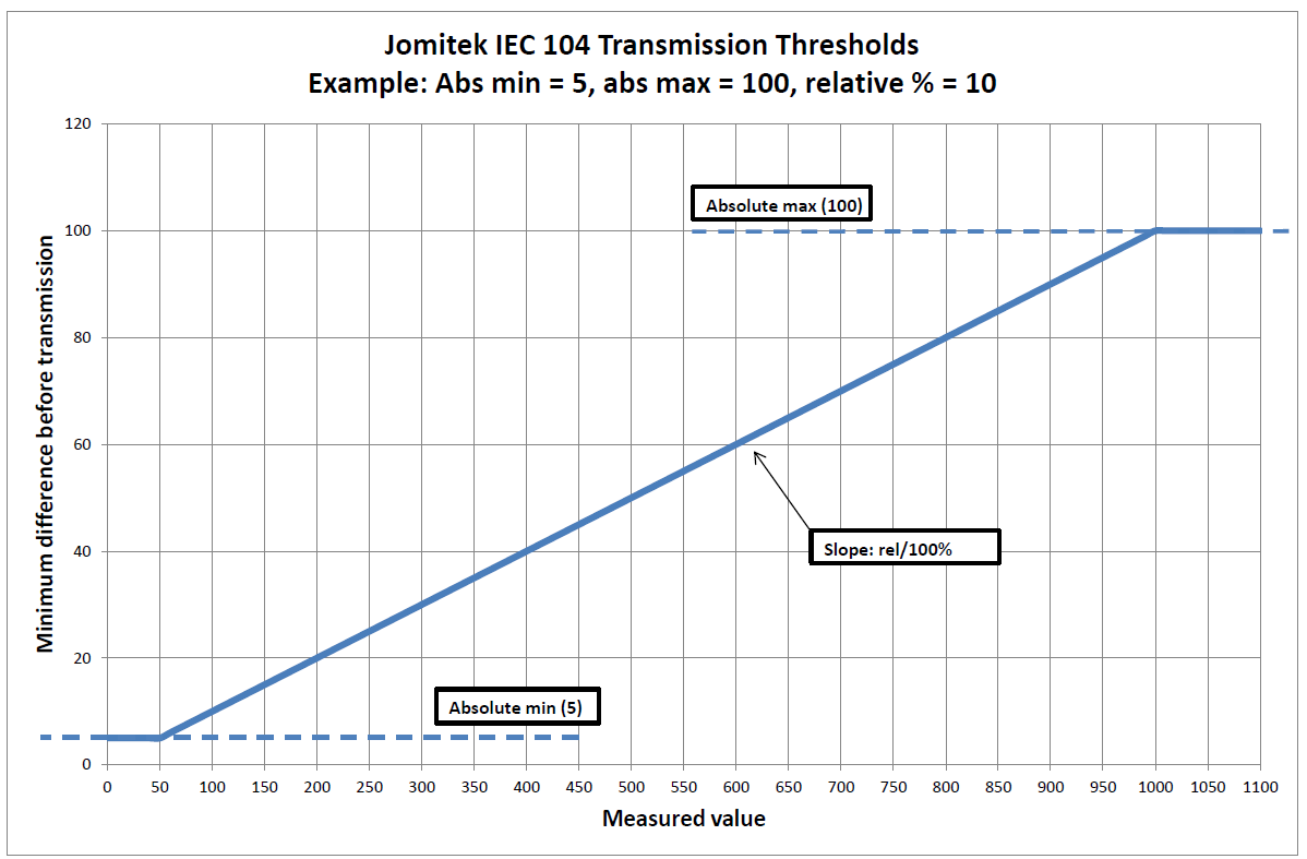
Figure 31: absmin, absmax and rel.
Any change in a digital value triggers transmission given spontaneous is set true for this data point in the “iec104_digital” sheet. For this reason the “iec104_digital” sheet does not define absmin, absmax and rel columns. Also, the “iec104_digital” sheet replaces the “cyclic” column found in the analogue sheet with “background”. The use of the “cyclic” column for analogue values is similar to the use of “background” column because they are both used to trigger transmission at fixed intervals.
Additionally, all IEC 104 commands are supported by the sensor, and they can be used to invoke any function or define any setting in the sensor as desired. However, depending on the application and due to the variety of protocols supported by the sensor, IEC 104 commands may not be needed. The “iec104_commands” sheet in the Excel file map a data point address to an internal variable.
Since the IEC 104 protocol uses TCP/IP, it is in some cases useful to debug the communication stream using Wireshark.
Updating sensor software
The software on the I3 sensor can be remotely updated in four simple steps:
- Download the newest update file from http://jomitek.dk/downloads/device_software_update
- Connect to the I3 sensor through the FTP interface with username service and password service1234.
- Transfer the update file, software.tar.gz, to the /service/software_update directory.
- Reset the I3 sensor through the web interface and wait for the update to apply.
The I3 sensor will now restart and apply the software update. It may be necessary to reconfigure the IP address of the sensor once the update is complete.
Efficient mass reconfiguration of sensors
The ‘conf/identity.conf‘ and ‘conf/settings.conf‘ files play a central role in the configuration and customization of a specific I3 sensor. It is vital to be able to update information for specific sensors across a range of sensors, or update a specific setting across all sensors without the need to retrieve, edit, and upload configuration files on a case by case basis.
These needs can be efficiently addressed using the Jomitek Mass Reconf Tool and underlying functionalities. In addition to the above mentioned .conf files, the I3 sensor continually checks for updates to these files in the form of a .reconf variant (‘identity.reconf‘ and ‘settings.reconf‘), which allows incremental update of specific parameters in the .conf files, without affecting the remaining parameters.
The end user may choose to use their own tools to generate Lua formatted ‘.reconf‘ files for large scale sensor management, or as an alternative use the functionality provided in the Macro enabled Excel sheets, which can be downloaded here (Excel 2007 or later) or here (Excel 97-2003).
Please read the User Manual-sheet in the Excel document carefully, and note the need for the WinSCP tool when distributing ‘.reconf” file updates automatically.
Measuring voltages
Measurement configurations
All voltage measurements use the sensor box grounding bolt as the reference level. It’s therefore important to ensure proper grounding of the sensor.
Starting with the most complete voltage measurement setup, an I3 Plus is used to measure 3 individual phase voltages, as well as e.g. a transformer star point voltage, or any auxillary voltage of interest in the measurement setup. In combination with current measurements, such a setup ensures a full overview on the power load, quality, and any fault situation on the individual phases measured.
A basic I3 sensor (or an I3 plus with only 1 input in use), allows for 1 voltage measurement point. The I3 sensor will automatically generate an internal copy of the remaining 2 phases, shifted 120 degrees to either side. This allows for a more cost efficient implementation, since the voltage measurement points can be be reduced to a minimum. This option allows for what would in many cases be a reasonable estimate of the reactive and active power load of the 2 phases with no direct voltage measurements. It is, however, not at setup which allows for full transparancy in e.g. situations with earth faults. The measurement limitations of such a setup should be weighed against the added installation costs of a full voltage measurement.
The I3 sensor can also be mounted on a current conducting cable with no voltage input. With no other I3 sensors locally, this will limit the measurement capabilities to be based on currents alone. This means that reactive and active power cannot be measured, as well as any type of directional measurement (e.g. direction of energy flow).
An option for synchronization of voltage measurements across several locally installed sensors (within the same LAN), is being researched by Jomitek, but is not commercially available yet. This option will help bring down installation cost on larger installations.
Voltage signal interfacing
The I3 sensors employ the same signal conditioning for all voltage inputs. The inputs are based on measurement via capacitive voltage division, and are protected up to 2kV. The high voltage capacity for a given nominal voltage should be selected such that:
Chv = 5×10⁴ [pF×V] / VnomRMS
This relation is translated into table 3:
| VnomRMS | Chv | Comment |
| 57.7 V (100 V/√3) | ≤820 pF | Standard output from voltage transformer |
| 110 V | ≤470 pF | 110 V RMS, as used in the US, low voltage |
| 230 V | ≤220 pF | 230 V RMS, as used in Europe, low voltage |
| 5.77 kV (10 kV/√3) | ≤8.6 pF | 10 kV RMS phase-phase, medium voltage level |
| 6.92 kV (12 kV/√3) | ≤7.2 pF | 12 kV RMS phase-phase, medium voltage level |
| 9.23 kV (16 kV/√3) | ≤5.4 pF | 16 kV RMS phase-phase, medium voltage level |
| 11.5 kV (20 kV/√3) | ≤4.3 pF | 20 kV RMS phase-phase, medium voltage level |
| 13.8 kV (24 kV/√3) | ≤3.6 pF | 24 kV RMS phase-phase, medium voltage level |
| 18.5 kV (32 kV/√3) | ≤2.7 pF | 32 kV RMS phase-phase, medium voltage level |
| 28.9 kV (50 kV/√3) | ≤1.7 pF | 50 kV RMS phase-phase, medium voltage level |
Table 3
Note that you may never make a direct galvanic connection to the voltage to be measured. You must always use a capacitor in between, appropriately selected based on above formula and table. Selecting a capacitor of much lower value than the maximum recommended, will reduce the dynamic range, and thus the measurement resolution of the nominal voltage. It is generally recommended to target a capacitor value no less than 25% of the maximum allowed value for a given voltage.
Jomitek produces a low voltage connector cable using a standard CEE interface, with integrated 220pF capacitors. This connector is part of the I3 Sensor Starter Kit, but can also be purchased in volume separately.
The maximum allowed capacitance value for the medium voltage levels fits well with industry standard silicone based capacitive test points, e.g. those found in elbow connectors. Note that ceramic based medium voltage capacitors should be avoided, as their capacity is both too high, and exhibits unlinear behavior as well. Note, that in order to obtain high accuracy voltage measurements, the capacitive test point must be screened, such that spread capacitances are avoided. Jomitek produces screening cups for elbow connectors. Please contact Jomitek for more information on medium voltage capacitive screening options.
Configuration of the capacity used, and further voltage scaling options are available in the ‘settings.conf’ file accessible via FTP or the sensor web interface.
A note on spread capacitances
In particular for the capacitors suitable for the medium voltage level, the physical distances involved between capacitor plates can lead to significant spread capacitances being introduced. Ideal solutions for such measurement systems involve well screened setups, such as using an elbow connector with integrated capacitive end plug, and placing a conducting screening cup as a termination for any parasitic/spread capacitances. This ensures that any capacitive coupling between the measurement plate and the surrounding material is constant, and preferably low compared to the capacitive coupling towards the medium voltage conductor.
In some cases it’s not possible to achieve a well screened solution at a reasonable cost. Non-ideal solutions may then be considered, at the cost of the usefulness of certain measurement parameters. Spread capacitances may lead to two main measurement deviation effects:
- Varying spread capacitance towards ground potential
- Cross talk between voltage phases
The first effect will change the capacitive voltage division ratio, leading to incorrect scaling of the voltage amplitude, and thus all measurement parameters related to the voltage amplitude. A typical example is with a setup where the unscreened medium voltage capacitor is near the enclosure door/lid of the installation. When opening the door, the spread capacitance to ground changes significantly, and thus the voltage division ratio. This effect may indicatively lead to 0-15% sensitivity variation.
The second effect is almost always experienced in combination with the first. It involves a capacitive coupling from one or more neighboring medium voltage conductors towards the measurement plate of the primary phase being measured. Effectively this results in the raw measurements of a given input being a mix of signals, with the major component being the primary phase measured, but with neighboring phases typically adding their signals at a 0-25% sensitivity level compared to the primary.
Cross talk between voltage phases can often be considered fairly static, as they are primarily dependent on the physical shape of a given type of breaker equipment. If the cross talk sensitivities have been mapped (calibrated) for a particular physical configuration, it can be reused on similar equipment models. It must however be confirmed that the enclosure is also fairly static, such that the first effect does not affect the second. One example of a measurement setup involving both spread capacitance measurement effects is on a Magnefix switchgear using a RetroCap measurement interface, as illustrated. In this case, the capacitive measurement point is glued to the surface of the fuses of a Magnefix switchgear. These are very easy to install, but unfortunately also very sensitive to cross talk and spread capacitances to ground.

Figure 32: Horstmann RetroCaps mounted on Magnefix switchgear.
Accuracy of measurement parameter vs. type of voltage measurement setup
| Measurement parameter | Well screened | Non-screened, specifically calibrated | Non-screened, calibrated by model | Non-screened, no de-mixing |
| phase_delta | OK | (OK) | Not OK | Not OK |
| phase_voltage | OK | (OK) | Not OK | Not OK |
| power_factor | OK | (OK) | Not OK | Not OK |
| rms_apparent_power | OK | OK | (OK) | Not OK |
| rms_reactive_power | OK | (OK) | Not OK | Not OK |
| rms_real_power | OK | (OK) | Not OK | Not OK |
| rms_voltage | OK | (OK) | (OK) | Not OK |
| thd_voltage | OK | OK | (OK) | (OK) |
Table 4: OK = Measurement will perform according to I3 data sheet specification,
(OK) = Measurement will likely perform according to I3 data sheet specification, but with no commitment from Jomitek,
Not OK = Measurement should be considered indicative at best, but with a high risk of being misleading
If the cross talk ratios have been determined, the I3 sensor platform supports on-the-fly de-mixing of the voltage measurement signals, effectively cancelling the cross talk phenomena. As suggested by the above table, it is strongly recommended to enable de-mixing of voltage cross talk, on installations with unscreened high voltage capacitors. Installation specific calibration will likely enable performance equal or close to a well screened system, but the cost of performing installation specific calibration will likely discourage such use cases. As such, installations will generally either be well screened, where needed, and otherwise non-screened, but calibrated according to the type (model) of the installation.
Guide for setting up voltage cross talk cancellation on the I3 sensor
Getting started
In order to enable the default cross talk cancellation settings, the following parameter should be set, either directly in the ‘settings.conf’ file or via the web interface: i3.calibration.voltage_cross_talk = true. IMPORTANT: Note that the interfacing to an I3 Plus must be symmetrical, i.e. of the following order: L1 I3 interface connected to either the top or bottom phase of the physical measurement setup, L2 to the center, and L3 opposite to the connection point of L1.
Advanced configuration and calibration
The cross talk figures provided per default are based on the behavior of a Magnefix switchgear. For other measurement setups, it is recommended to verify that the same cross talk relation applies, and if not, the cross talk parameters must be updated to reflect the behaviour of the relevant measurement setup. These parameters can be found in the i3.calibration.voltage_cross_talk_coeff folder. Using the web interface, the subfolder L1 reflects the relative signal strengths received on L1 from the phase connected to L1 (denoted phase01), L2 (phase02), L3 (phase03) and the auxillary input (phase04) respectively. The same logic applies for the remaining subfolders. It is the same reference input level used across all the calibration measurements. It is recommended to use the L2 input, when applying a reference voltage signal to the phase of L2 capacitor, as the mentioned reference.
As an example, figure 33 illustrates a case where
- A reference voltage was applied to the phase being interfaced to L2 on the I3, while the other phases were kept grounded, and the resulting output noted for the L2 input. This is the reference input level the following measurements was normalized with, and it is with respect to this level, that the i3.voltage_setup.phase02_hv_capacitor value was aligned, such that the absolute voltage measured by the I3 matches that of the known voltage level of the reference voltage.
- The same reference signal was then applied to the phase being interfaced to L1, L2 and L3, one at a time, and with the other phases grounded for each measurement. The input on L1 was normalized with respect to the first measurement, and a signal strength of 127.0%, 11.2% and 3.0% was noted.
- The auxillary input was not connected, so the cross talk for AUX is set to 0%.
- The AUX input, is assumed free of cross talk and therefore indicated with 0% for cross talk from signals relating to L1-L3.
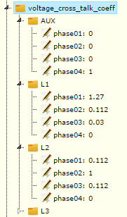
Figure 33
Following the guideline above, a capacitance value of 3.2 pF was found for the Horstmann RetroCap sensors mounted on a Magnefix switchgear. This value must be specified in i3.voltage_setup.phase0[x]_hv_capacitor, with [x] being 1-3.
Troubleshooting
The I3 starter kit includes one year of free e-mail support.
Please direct all questions to the Jomitek support engineers by emailing to support@jomitek.dk.
Appendix
Web interface menu structure
For manual configuration and testing purposes, as well as functionality verification, the I3 sensor comes with a web server offering a simple GUI.
- Reset options performs a full reset of the device, which will restart the processor, and reload all configuration files.
- Settings provides a web based overview and modification option for the ‘conf/settings.conf‘ file.
- Identity provides a web based overview and modification option for the ‘conf/identity.conf‘ file.
- Device state, is a web based overview of the main data table (database), which is generated via the framework found in the ‘conf/data.conf’.
- Download measurement snapshots presents a view of links to ‘.wav‘ files found in the ‘web/m/‘ folder in the RAM part of the file system (volatile data).
- View measurement snapshots presents the content of the ‘.wav‘ files mentioned above, with a simple web based graph tool.
- Live measurements may be used to view live updated values for select parameters in the main data table, using a simple web based graph tool.
Starting from the top of the default I3 sensor main web page:
A map (loaded from client-side) and address information can be toggled using the link in the top right corner, ‘See location information‘. The intended purpose, is to make sure that the sensor location can be identified by the sensor itself, and easily visualized. The source data is extracted from the ‘conf/identity.conf‘ file. For the full address string, the fields address, city, zip, and country_state are used. For the map, the WGS84 coordinates must be entered in the format ‘<latitude>,<longitude>’ in decimal degrees, e.g. ‘55.822051, 12.488554’.
Below the location information link the main information view is presented using a tree view structure with information ‘folders’ which can be expanded. Depending on the information type, the lowest level expansion will either act as a button executing the relevant command, a link for file download, a link which expands the bottom part of the main page with the requested content, or in case of specific parameter values, the value is inserted in an editable text box.
The main folder (top level icon) represents the I3 Sensor device itself, including a few main status and identification parameters. The device text is assembled using the following parameters: The ‘type’ and ‘serial_number’ from ‘conf/identity.conf‘, the MAC address using a special system call and the processor core temperature using another system call. When the mouse cursor is positioned on the folder, additional information presenting the server side time (GMT) of the web page load will occur.
The Reset options features a Reset main device button. A reset command is sent to the sensor, and the web client is set to automatically reload the page when the sensor should be up and running again. If this is not the case, please reload the page again, and remember to check that the IP address targeted is still correct after the reset.
The Settings information folder presents a database table as defined by the ‘conf/settings.conf‘ file. Any web based modication of the parameters will be directly updated in the .conf file itself. Note that most parameter changes will require a reset to take effect. This folder, along with the Identity and Device state folders, is a direct mapping of a data table in Lua (in this case ‘CONFIG’). This is the reason why there are no ‘space’ characters, or other special characters, in the subfolder and parameter names. It provides the added benefit, that any modification in the Lua data tables will be directly reflected on the web page at the next reload.
Note that the majority of the parameters in the Settings folder are described by placing the cursor above the parameter in question. The same is the case for many of the parameters included in the other folders. The descriptions, as well as basic data format validation during web based parameter updates, are per default defined via the ‘conf/description.csv” file, or in the iec104 data point mapping .csv files, e.g. ‘conf/iec104_analogue.csv‘.
The database subfolder defines a few high level behavior settings for the main Lua data table.
The i3 subfolder contains a number of I3 Sensor specific configuration options:
- calibration is offering a simple linear scaling option for current and voltages. It is only expected to be needed for fine tuning of voltages. An option for a general adjustment of the voltage to current phase is also offered, but should only be used if trustworthy reference measurements have shown it to be necessary. This could be the case, if the currents are measured at the MV side of a transformer, and the voltages are from the LV side.
- estimator defines the high level settings for the position estimation algorithm. By clicking on the folder icon, a special view is triggered. This expands the bottom of the main page to include a simple schematic of the I3 Sensor (the small version per default), including position estimates for the first 4 conductors in the model. This view can be used as a basic sanity check, to confirm that the estimator has arrived at a reasonable result. The absolute_threshold, relative_threshold, and the timer fields define the criteria for starting a new position estimation cycle. The two first acts on the estimator error (Device state ⇒ state ⇒ estimator_error), while the last is a cyclic timer. The estimator_mode defines the geometry type, that the estimator is using. Clicking on this parameter triggers a special view which presents a table with schematics of all the applicable modes. Clicking on a schematic will automatically change the model used. The results should then be visible after the following position estimation cycle.
- event_settings defines trigger points for logging of measurement events.
- phase_identification provides a settings list for naming and linking of the currents measured.
- post_processing defines processing steps related to the RMS calculations performed on the raw measurement data. flip_direction_of_current (default: false) can be used to reverse the sign of the current, and hereby flip the sign of the active power measurement (direction of energy flow). Note that with the default setting (false) a positive active power flow is defined as being fed from the bottom (where the lid of the I3 sensor is mounted), to the topside (the blank surface). The RMS readout of measurement values are split up into two dimensions. The first, defined by quick_time, is intended to provide near-instantaneous true RMS measurements for use in the web interface. The default setting is 1 second. The second, defined by average_time is intended to provide true RMS averaging windows for SCADA/automated readouts, with a default setting of 60 seconds.
- voltage_setup defines the high voltage capacity, in pF, used for the voltage measurement. Lua background processing translates the value into an appropriate scaling factor used internally in the sensor system.
iec104 lists all main parameters used for the IEC 60870-5-104 protocol configuration, including file links used for address mapping and type definition of parameters.
logging provides parameterization options for what event or error types should be put into the system log. See also /log via FTP. In general, it should not be needed to change these settings.
tcpip provides the option whether to use dhcp or not. Per default dhcp is set to true. The IP and gateway adresses and the subnet mask is also defined here (only used if dhcp=false). Note that if the device experiences severe errors during startup, it will revert to the IP configuration defined in the ‘conf/panic.ip‘ file, and if this also fail to load, the following hardcoded settings will be used: dhcp=false, gateway=192.168.135.100, ipv4=192.168.135.18, subnet=255.255.255.0. In DHCP mode, in the case where no DHCP server can be reached, the sensor will automatically make an allocation within the IP range 169.254.1.0 to 169.254.254.255 in compliance with RFC 3927 Section 2.1.
The parameters in the web section defines which port is used for the web service (default is ’80’), and the file path for the description file used to link in (a) basic parameter validation via the web interface (‘boolean’, ‘integer’, ‘float’, ‘string’, ‘ipv4’), and (b) description text when mouse cursor is above the parameter in question.
The Identity folder contains all the location and naming related information for a specific device. It should always be edited, or generated, on an individual basis. The parameters include address, city, zip, country_state, location_name and location_description as identifying text for the location. The location_name could e.g. be the name or reference for a substation, and the location_description could detail the cable section and/or phases being measured on. Furthermore the location may be specified using WGS84 coordinates in a ‘<latitude>,<longitude>’ decimal degrees format, as earlier mentioned. The serial_number may be set to match the Jomitek device serial number, or a custom format defined by the operator. In this context, note that the only hardcoded identifier of a device is the uniquely assigned MAC address. The type parameter will, if left blank, be automatically set at run time based on a device internal check of the accessible peripherals. Custom naming may be used as an alternative.
The Device state reflects the ‘data’ Lua table. It contains a measurement data hierachy starting with measurement nodes; 1 for each of the 4 phases possible to measure as main sources, and a post-processing summary on the section level (average and aggregation, where relevant, of measurement values for phases 1-3). Below each measurement node the following list of measurement parameters are reflected:
- phase_current is the phase, in degrees, of the current with respect to the sensor master reference, which is typically the voltage input belonging to phase01.
- phase_delta is the phase difference, in degrees, between the paired voltage and current of a given phase. A leading voltage is defined as positive.
- phase_voltage is the phase, in degrees, of the voltage with respect to the sensor master reference, which is typically the voltage input belonging to phase01.
- power_factor is the power factor, defined as the active power, P, divided by the apparent power, S.
- rms_apparent_power is the apparent power (current RMS multiplied with voltage RMS), in kVA.
- rms_current is the RMS current, in A.
- rms_reactive_power is the reactive power, in kVAr.
- rms_real_power is the real (active) power, in kW.
- rms_voltage is the RMS voltage, in kV.
- thd_current is the Total Harmonic Distortion of the current.
- thd_voltage is the Total Harmonic Distortion of the voltage.
Except for the THD measurements all of the above values are based on the ‘CONFIG.i3.post_processing.average_time’ RMS averaging window. The THD measurements are based on the latest frequency analysis (hardcoded to run for all active voltage and current inputs, once every 10 minutes).
For the section measurement node, phase measurements are not applicable, but otherwise the same parameters as mentioned above can be found. In addition the ‘main_harmonic_frequency’ of the master measurement channel (default is voltage of phase 01).
In addition to the phase and section measurement nodes, a ‘state’ node displays the status for the sensor unit.
- estimator_error is an error figure result from the last completed physical position estimation of the phases
- mac_address may be used to provide unique identification of the sensor unit
- resource_alert is 1, when either the RAM or flash dips below 1MB of free memory or the processor load is 100% for 10 consecutive cycles.
- processor_temperature is the processor temperature in degrees Celcius. The temperature should remain below 75 degrees in normal operation. This measure may be used to indicate the temperature of the conductor as well, depending on the mounting conditions.
Conductor models
The I3 sensor needs a model of the physical conductor configuration to estimate current. Pick the correct model from the overview presented below and set it in the web interface.
 |
|
| Primary conductor. | |
| External conductor. | |
| Exclusion zone. No conductors or ferromagnetic materials. | |
| Primary conductor zone. | |
| Sensor casing. |
Figure 34: Conductor model legend.
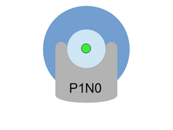 Figure 35: Single conductor. |
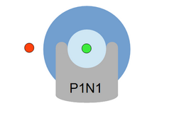 Figure 36: Single conductor with one external conductor. |
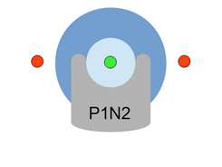 Figure 37: Single conductor with two external conductors. |
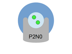 Figure 38: Two conductors. |
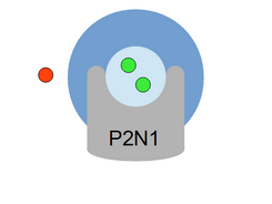 Figure 39: Two conductors with one external conductor. |
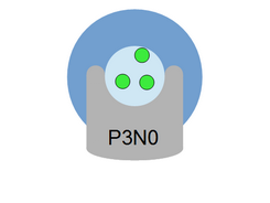 Figure 40: Three conductors with arbitrary geometry. |
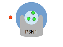 Figure 41: Three conductors with arbitrary geometry and one external conductor. |
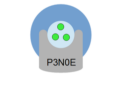 Figure 42: Three conductors with equilateral geometry. |
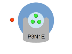 Figure 43: Three conductors with equilateral geometry and one external conductor. |
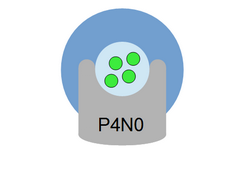 Figure 44: Four conductors with arbitrary geometry. |
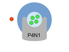 Figure 43: Four conductors with one external conductor. |
 Figure 45: Four conductors with equilateral geometry. |
 Figure 46: Four conductors with equilateral geometry and one external conductor. |
Telnet commands
- help
- cd <dir>
- cdrive <num>
- tasks
- cat <file>
- mv <old> <new>
- rm <name>
- mkdir <dir>
- getfree
- format <num> <format>
- pwd
- ls <[dir]>
- reset
help
– Show a list of Telnet commands.
cd <dir>
– Change directory to <dir>
cdrive <num>
– Change drive number.
tasks
– Show a list of running tasks.
cat <file>
– Show the contents of a file.
mv <old> <new>
– Move or rename a file or directory.
rm <name>
– Delete a file or directory.
mkdir <dir>
– Create a directory <dir>
getfree
– Get sixe of free space in drive <[num]>.
format <num>
– Format drive <num>.
pwd
– Show the current working directory.
ls <[dir]>
– List contents of current working directory or <[dir]>.
reset
– Restart the I3 sensor.